I’ve lived in several different parts of the world, and they all do internet differently. Back in the US I had 8Mb/sec cable (leaving just before Fios was really an option, darn!) In New Zealand, for instance, I was paying for “high speed ADSL” rated at 1.5Mb/256k. Vrooom. Up in Taiwan I was paying 1/2 what I paid in New Zealand, but for 12Mb/1Mb. Down to Sydney and we have a rated 24Mb/1Mb.

But there’s a catch with the plans in New Zealand and Australia: they are ‘capped’. This means you only get XGB/month – and it isn’t like Comcast capping at 250GB/month, I’m talking about 1GB/5GB/10GB and so forth. And there’s more – just like mobile phones, you get on-peak and off-peak times.

This all does make a bit of sense to me – there are only X amount of tubes going in and out of NZ and AU, and I would imagine they get pretty clogged.

Either way, last month was pretty painful. Two weeks into our plan I checked out usage: 14GB of 18GB! We had only 4GB left to use for 15 days. This sounds like a lot, but for the two of us, and my 10 virtual servers, it isn’t. The first thing I did was looking at a way to do WSUS with Linux – I ended up using apt-cacher (I’m using only Ubuntu at home). BitTorrent, out; downloading any new ISOs, out; streaming music, totally out. For a while I has to VPN to home, and then VPN to a client, as our router at work didn’t seem to like letting us access one of our clients. I even disconnected from the VPN if I wouldn’t be doing work for 20m!

We eventually made it, and used only 2GB in two weeks. What an accomplishment!

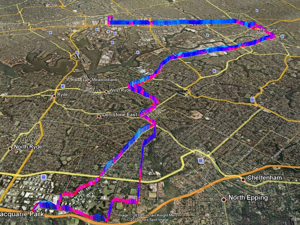
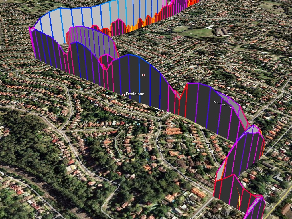
I showed a few of my co-workers my graph and one replied – oh! that’s really cool. (I think only two of my co-workers are actually interested in my geekyness). He then emailed me tonight a .kmz file containing a colorized file of his speed. I looked at the kml and noticed it appeared to be dynamically allocated judging by the top speed. Well, as you could guess, I surely had to modify my code to include colors.

Within an hour I had a semi-working example, and within two hours will easily be done with this blog post. The code might not be perfect, but it first parses the xml and returns the max speed for the trip. Next, it colorizes the speeds based on a scale of 0-255, with 0 being blue for fast and 255 for being yellow, or slow. I was going to study for the CCNA tonight, but it looks like writing Python is just too much fun.

So what, you might ask, are those dips? Good question. They are huge speed bumps (and the tall blue mound in the middle is a really steep hill).

I recently have been playing with parsing GPX files and spitting out the results into a special KML file. I initially wrote a parser using minidom, yet after running this the first time – and my Core2Duo laptop reaching 100% utilization for 10 seconds – I realized I needed to re-write it using something else.

I spent a little time reading the different parsers for XML and eventually read more about cElementTree. And it is included with Python2.5, sweet.

I quickly rewrote the code and did some tests. First, the two bits of code for parsing my GPX file:

minidom-speed.py

#!/usr/bin/python

from xml.dom import minidom
from genshi.template import TemplateLoader

def collect_info():
dom = minidom.parse('airport.gpx')
for node in dom.getElementsByTagName('trkpt'):
lat = node.getAttribute('lat')
lon = node.getAttribute('lon')
speed = node.getElementsByTagName('speed')[0].firstChild.data
speed = float(speed) * 10
coords = '%s,%s' % (lon, lat)
coords_speed = '%s,%s' % (coords, speed)
yield {
'coordinates': coords_speed
}

loader = TemplateLoader(['.'])
template = loader.load('template-speed.kml')
stream = template.generate(collection=collect_info())

f = open('minidom.kml', 'w')
f.write(stream.render())

cet-speed.py

#!/usr/bin/python

import sys,os
import xml.etree.cElementTree as ET
import string
from genshi.template import TemplateLoader

def collect_info():
mainNS=string.Template("{http://www.topografix.com/GPX/1/0}$tag")

wptTag=mainNS.substitute(tag="trkpt")
nameTag=mainNS.substitute(tag="speed")

et=ET.parse(open("airport.gpx"))
for wpt in et.findall("//"+wptTag):
wptinfo=[]
wptinfo.append(wpt.get("lon"))
wptinfo.append(wpt.get("lat"))
wptinfo.append(str(float(wpt.findtext(nameTag)) * 10))
coords_speed = ",".join(wptinfo)
yield {
'coordinates': coords_speed,
}

loader = TemplateLoader(['.'])
template = loader.load('template-speed.kml')
stream = template.generate(collection=collect_info())

f = open('cet.kml', 'w')
f.write(stream.render())

The speed difference is not just noticeable, but very noticeable.

minidom-speed.py

$ python -m cProfile minidom-speed.py
4405376 function calls (3787047 primitive calls) in 32.142 CPU seconds

cet-speed.py

$ python -m cProfile cet-speed.py
1082061 function calls (904167 primitive calls) in 6.736 CPU seconds

A quarter as many calls and almost 5x faster – at least that’s how I interpret the results. Much better!